Asset metadata as Markdown

In Lesson 9, you created the adhoc_request asset. During materialization, the asset generates and saves a bar graph to storage. This setup is great for referring to the chart at a later time, but what about what’s generated right after a materialization? By using metadata, you can view the chart right in the Dagster UI!

Adding the metadata to the asset

1. Navigate to and open assets/requests.py.

2. At this point in the course, the adhoc_request asset should look like this:

   import dagster as dg
   from dagster_duckdb import DuckDBResource
   
   import matplotlib.pyplot as plt
   
   from dagster_essentials.assets import constants
   
   class AdhocRequestConfig(dg.Config):
     filename: str
     borough: str
     start_date: str
     end_date: str
   
   @dg.asset
   def adhoc_request(config: AdhocRequestConfig, taxi_zones, taxi_trips, database: DuckDBResource) -> None:
       """
         The response to an request made in the `requests` directory.
         See `requests/README.md` for more information.
       """
   
       # strip the file extension from the filename, and use it as the output filename
       file_path = constants.REQUEST_DESTINATION_TEMPLATE_FILE_PATH.format(config.filename.split('.')[0])
   
       # count the number of trips that picked up in a given borough, aggregated by time of day and hour of day
       query = f"""
           select
             date_part('hour', pickup_datetime) as hour_of_day,
             date_part('dayofweek', pickup_datetime) as day_of_week_num,
             case date_part('dayofweek', pickup_datetime)
               when 0 then 'Sunday'
               when 1 then 'Monday'
               when 2 then 'Tuesday'
               when 3 then 'Wednesday'
               when 4 then 'Thursday'
               when 5 then 'Friday'
               when 6 then 'Saturday'
             end as day_of_week,
             count(*) as num_trips
           from trips
           left join zones on trips.pickup_zone_id = zones.zone_id
           where pickup_datetime >= '{config.start_date}'
           and pickup_datetime < '{config.end_date}'
           and pickup_zone_id in (
             select zone_id
             from zones
             where borough = '{config.borough}'
           )
           group by 1, 2
           order by 1, 2 asc
       """
   
       with database.get_connection() as conn:
           results = conn.execute(query).fetch_df()
   
       fig, ax = plt.subplots(figsize=(10, 6))
        
       # Pivot data for stacked bar chart
       results_pivot = results.pivot(index="hour_of_day", columns="day_of_week", values="num_trips")
       results_pivot.plot(kind="bar", stacked=True, ax=ax, colormap="viridis")
   
       ax.set_title(f"Number of trips by hour of day in {config.borough}, from {config.start_date} to {config.end_date}")
       ax.set_xlabel("Hour of Day")
       ax.set_ylabel("Number of Trips")
       ax.legend(title="Day of Week")
   
       plt.xticks(rotation=45)
       plt.tight_layout()
   
       plt.savefig(file_path)
       plt.close(fig)
   

3. Add the base64 import to the top of the file:

   import base64
   import dagster as dg
   

4. After the last line in the asset, add the following code:

   with open(file_path, 'rb') as file:
       image_data = file.read()
   

5. Next, we’ll use base64 encoding to convert the chart to Markdown. After the image_data line, add the following code:

   base64_data = base64.b64encode(image_data).decode('utf-8')
   md_content = f"![Image](data:image/jpeg;base64,{base64_data})"
   

6. Finally, we'll return a MaterializeResult object with the metadata specified as a parameter:

   return dg.MaterializeResult(
       metadata={
           "preview": dg.MetadataValue.md(md_content)
       }
   )
   

   Let’s break down what’s happening here:

   1. A variable named base64_data is created.
   2. base64.b64encode encodes the image’s binary data (image_data) into base64 format.
   3. Next, the encoded image data is converted to a UTF-8 encoded string using the decode function.
   4. Next, a variable named md_content is created. The value of this variable is a Markdown-formatted string containing a JPEG image, where the base64 representation of the image is inserted.
   5. To include the metadata on the asset, we returned a MaterializeResult instance with the image passed in as metadata. The metadata will have a preview label in the Dagster UI.
   6. Using MetadataValue.md, the md_content is typed as Markdown. This ensures Dagster will correctly render the chart.

At this point, the code for the adhoc_request asset should look like this:

import dagster as dg
from dagster_duckdb import DuckDBResource

import matplotlib.pyplot as plt
import base64

from dagster_essentials.assets import constants

class AdhocRequestConfig(dg.Config):
    filename: str
    borough: str
    start_date: str
    end_date: str

@dg.asset
def adhoc_request(config: AdhocRequestConfig, database: DuckDBResource) -> dg.MaterializeResult:
    """
      The response to an request made in the `requests` directory.
      See `requests/README.md` for more information.
    """

    # strip the file extension from the filename, and use it as the output filename
    file_path = constants.REQUEST_DESTINATION_TEMPLATE_FILE_PATH.format(config.filename.split('.')[0])

    # count the number of trips that picked up in a given borough, aggregated by time of day and hour of day
    query = f"""
        select
          date_part('hour', pickup_datetime) as hour_of_day,
          date_part('dayofweek', pickup_datetime) as day_of_week_num,
          case date_part('dayofweek', pickup_datetime)
            when 0 then 'Sunday'
            when 1 then 'Monday'
            when 2 then 'Tuesday'
            when 3 then 'Wednesday'
            when 4 then 'Thursday'
            when 5 then 'Friday'
            when 6 then 'Saturday'
          end as day_of_week,
          count(*) as num_trips
        from trips
        left join zones on trips.pickup_zone_id = zones.zone_id
        where pickup_datetime >= '{config.start_date}'
        and pickup_datetime < '{config.end_date}'
        and pickup_zone_id in (
          select zone_id
          from zones
          where borough = '{config.borough}'
        )
        group by 1, 2
        order by 1, 2 asc
    """

    fig, ax = plt.subplots(figsize=(10, 6))
    
    # Pivot data for stacked bar chart
    results_pivot = results.pivot(index="hour_of_day", columns="day_of_week", values="num_trips")
    results_pivot.plot(kind="bar", stacked=True, ax=ax, colormap="viridis")
    
    ax.set_title(f"Number of trips by hour of day in {config.borough}, from {config.start_date} to {config.end_date}")
    ax.set_xlabel("Hour of Day")
    ax.set_ylabel("Number of Trips")
    ax.legend(title="Day of Week")
    
    plt.xticks(rotation=45)
    plt.tight_layout()
    
    plt.savefig(file_path)
    plt.close(fig)

    with open(file_path, "rb") as file:
        image_data = file.read()

    base64_data = base64.b64encode(image_data).decode('utf-8')
    md_content = f"![Image](data:image/jpeg;base64,{base64_data})"

    return dg.MaterializeResult(
        metadata={
            "preview": dg.MetadataValue.md(md_content)
        }
    )

Viewing the metadata in the Dagster UI

After all that work, let’s check out what this looks like in the UI!

1. Navigate to the Global Asset Lineage page.
2. Click Reload definitions.
3. After the metadata code is updated, simulate a tick of the sensor.

On the right-hand side of the screen, you’ll see preview, which was the label given to the Markdown plot value:

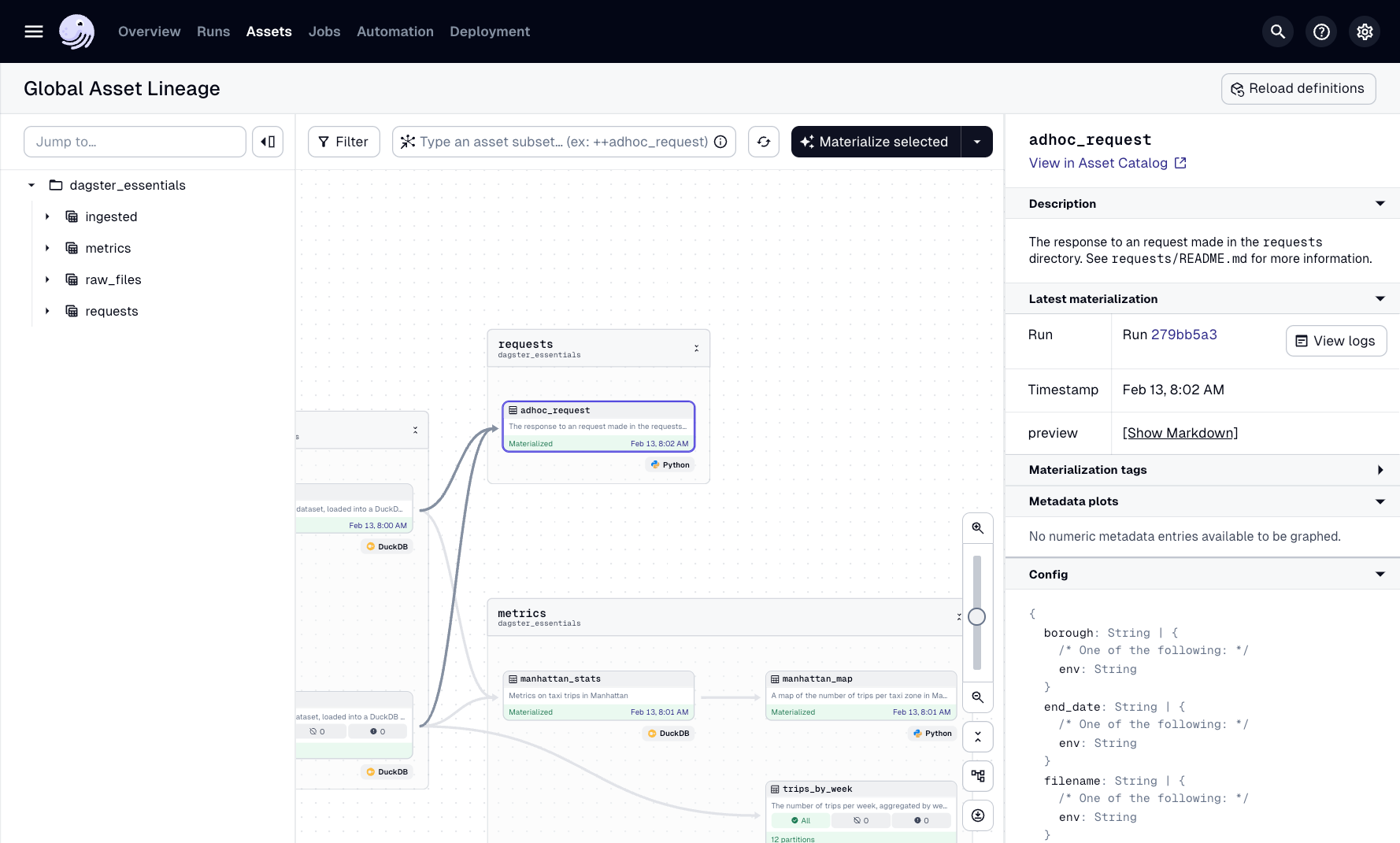
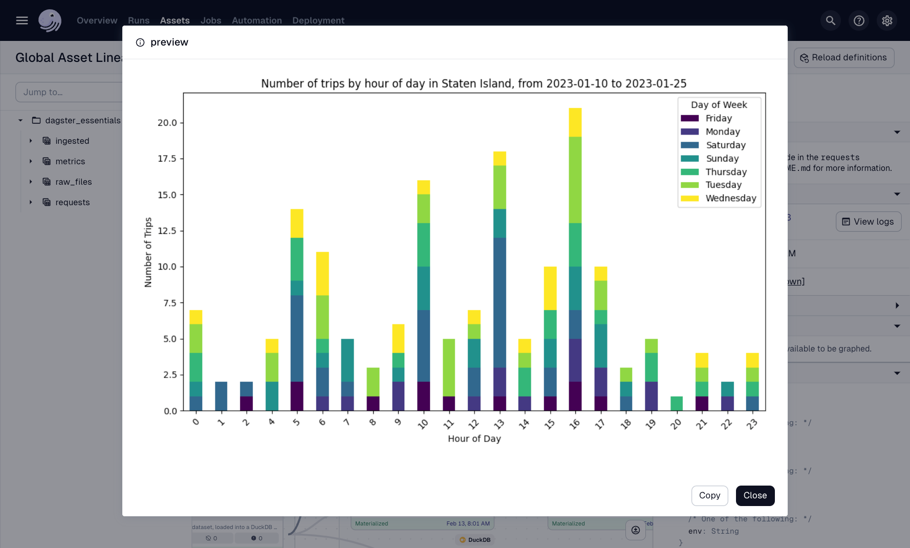
To display the chart, click [Show Markdown] :

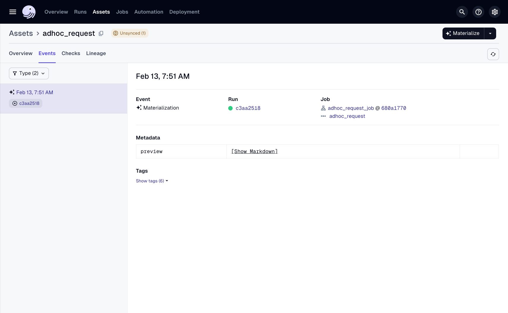
You can also click View in Asset Catalog to view the chart: